800,000 #InaugurationDay Tweets - Preliminary Analysis

Yesterday, Donald Trump has been inaugurated as the President of USA… However, this post is not, at least not directly, about Donald Trump, but about what was happening on Twitter during #InaugurationDay.

For the last few weeks I have been working on new tweet collection software called TweetPinna (soon to be open sourced available on GitHub). Thinking about the inauguration, I decided to do a little stress test. This resulted in a database filled with 789,051 tweets, spread over a period of ten hours. Unfortunately, due to the Twitter ToS, I cannot share the (anonymized) raw data. However, if you want to play with the data, I can provide you with all twitter IDs and necessary instructions.

Since these tweets seems to be very interesting, I decided to have a (very) preliminary look into the data.

General Information / EDA

The collection software ran between Fri, 20 Jan 2017 15:49:48.187 GMT and Sat, 21 Jan 2017 00:38:48.670 GMT. Overall, 789,051 tweets were collected and stored in a MongoDB collection.

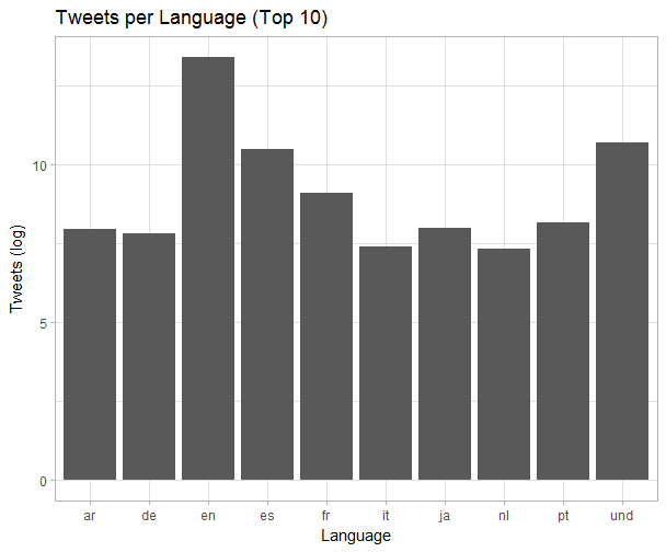
Based on metadata, there are tweets in 53 different languages in the collection. The languages with the highest frequencies of tweets are listed below:

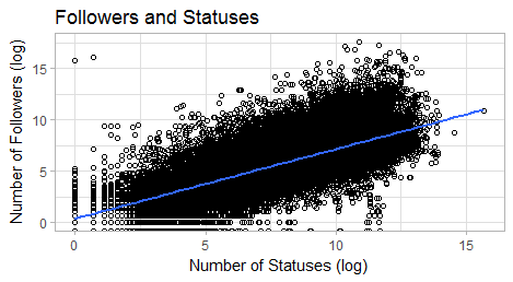
The data also is interesting regarding the people involved. As we can see in this plot, there is a fairly strong correlation between the number of statuses and the number of followers.

Hashtags

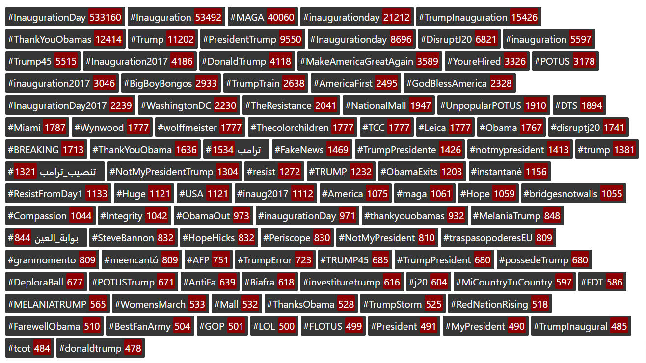
There are 18589 unique hashtags (948,833 in total; avg. of 1.2 hashtags per tweet) in the collection. Since #InaugurationDay was the starting point of the collection process, it clearly is the most frequent hashtag/item in the collection.

The most prominent hashtags are:

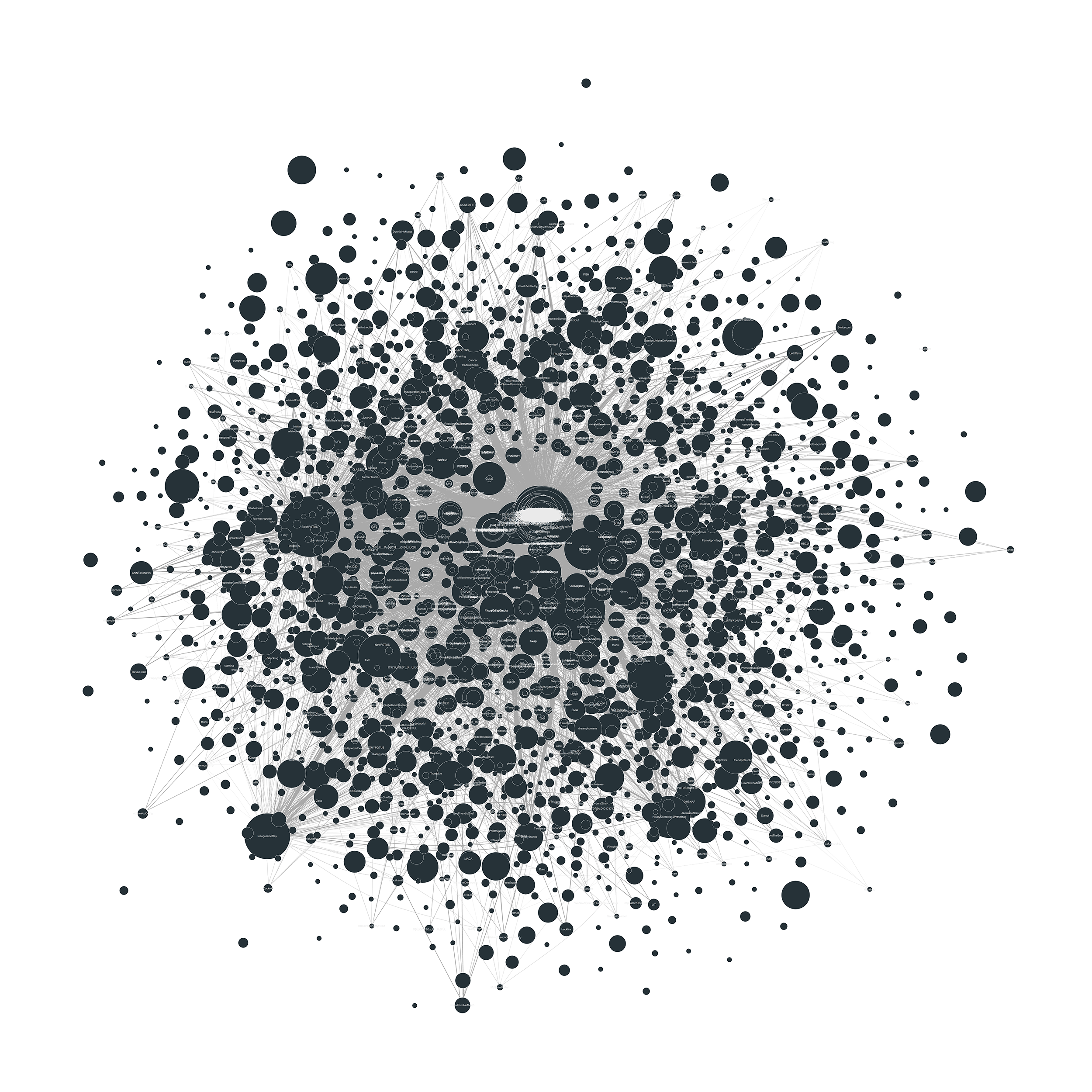
Plotting hashtag co-occurence as a network plot results in a rather beautiful, but crowded picture. Nodes that are connected have appeared together in a tweet. The size of the node represents the number of total occurences.

In order to actually see something, the sample size needs to be reduced. The following graph shows a sample of 1000 tweets and their respective hashtags.

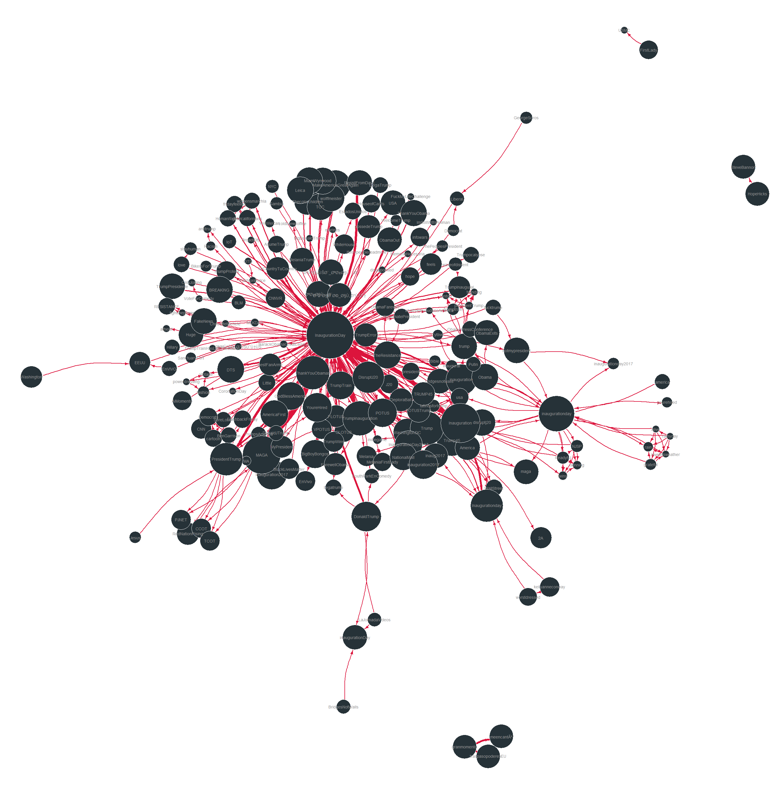
The network plot was generated using the Fruchterman-Reingold algorithm (niter = 10,000) in igraph. The size of the nodes represents the overall frequency of the hashtags in the collection. The width of the edges represents the number of co-occurences in the sample. Isolated hashtags have been removed. Still, there are three isolated groups of hashtags in the sample. These most often represent individual tweets with multiple hashtags that are not used by other tweets.

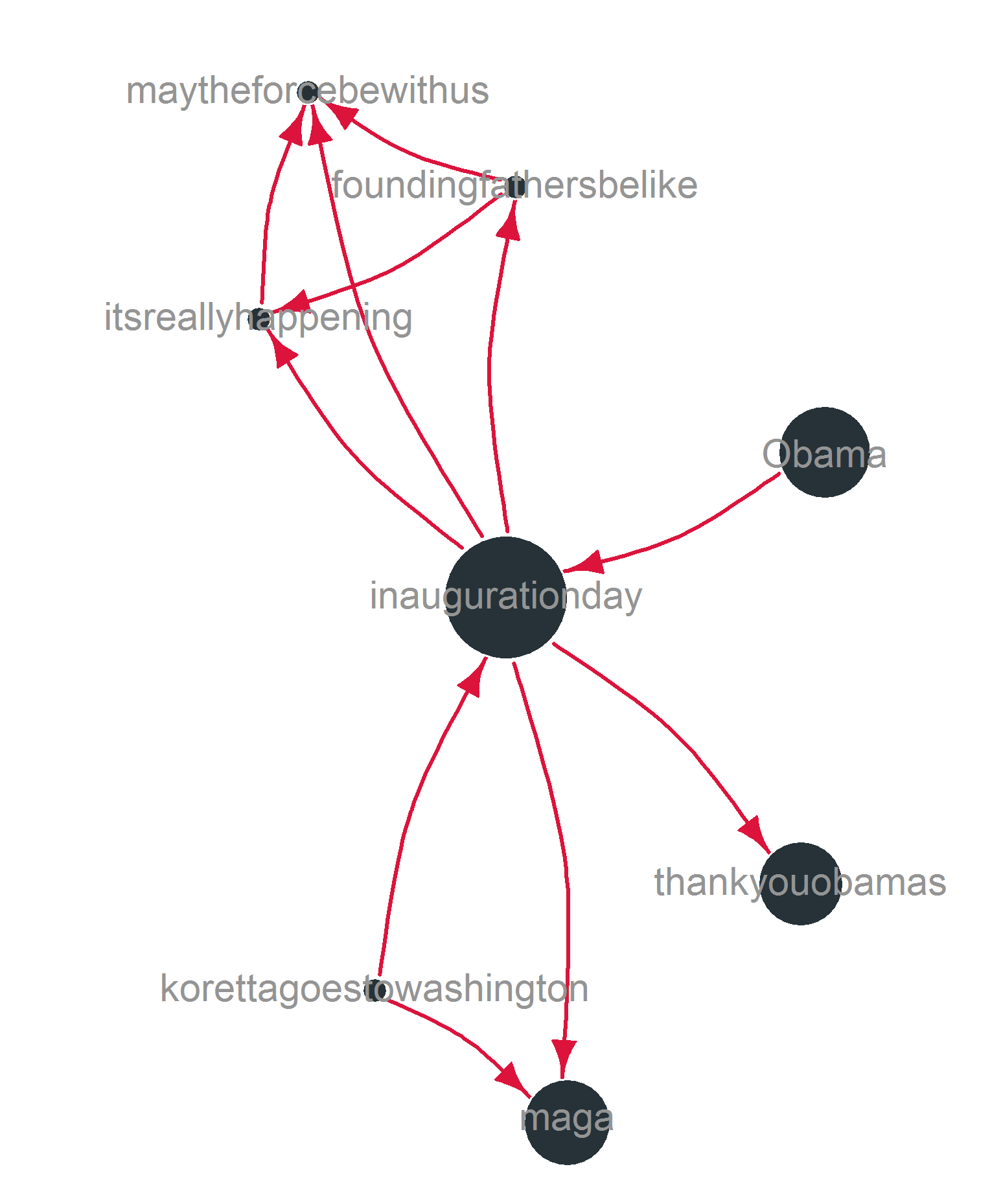
This individual, non-representative configuration of hashtags (from a sample of 100 tweets) reveals how different discourses are linked by central nodes (more general hashtags) in the network. In this particular example a set of critical hashtags consisting of maytheforcebewithus, foundingfathersbelike, and itsreallyhappening is linked to the larger discourse using the general inaugurationday hashtag.

Unfortunately, I have not yet undertaken any further, in-depth, analysis.

Corpus of English Tweets

I decided to primarily focus on original English tweets. Hence, the actual corpus is a subset of the collection consisting of English tweets which are not marked as a retweet. This has been achieved by querying MongoDB db.getCollection('inaugurationday').find({text: {$not: /^RT.*/}, lang: "en"}). This fairly simple regex methodology (i.e. excluding tweets starting with ‘RT’) is not perfect, but works well enough. The actual tweets were then extracted from the databse using a simple Python script creating a csv file that can easily be processed using R. Actually, most of the data wrangling, analysis, and visualization has been done in R.

Following this process resulted in a list of 133,618 English tweets. Due to a lack of computing power (yes, with this amount of data this becomes an issue), I drew a random sample of 10,000 tweets (= 44,687 tokens) that I will use for parts of the analysis.

I cleaned the tweets using both tweet_utils (@timothyrenner) and the various tm_map functions. To exclude stopwords, the SMART list was used.

Frequency

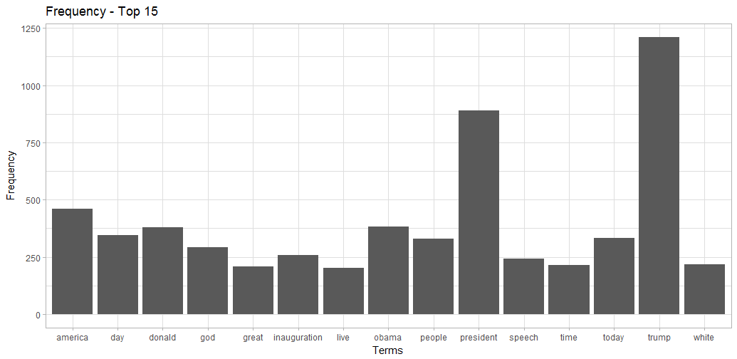
Overall, the frequency plot does not reveal anything particularly interesting. Nevertheless, it becomes clear that both Presidents (Obama and Trump) are discussed in the inauguration context. Comparing these results to a similar frequency analysis of the whole dataset revealed that random sampling worked really well.

Looking at the frequencies over time (absolute frequency per hour) is more fruitful. I have removed some of the omnipresent, high-frequency terms (‘trump’, ‘america’, ‘american’, ‘day’, ‘president’, ‘obama’, ‘today’, ‘god’, ‘donald’, ‘people’) in order to foreground some of the less frequent words.

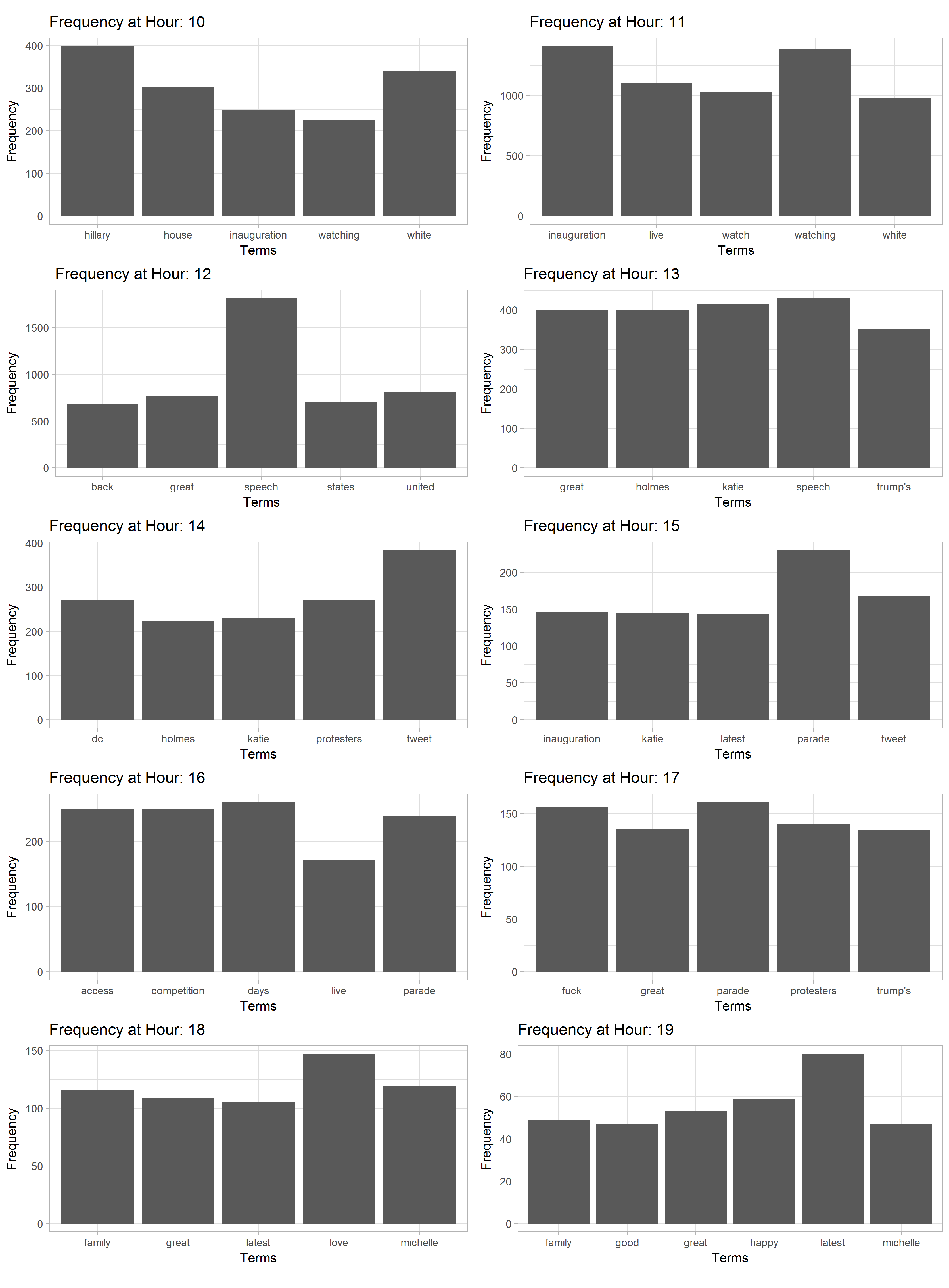
The frequencies reveal a fair bit of information about what was going on. For example, the appearance of Katie Holmes, Trump’s speech, and the 3pm Parade are clearly visible in the data.

The term ‘inauguration’ was only highly frequent during the first two hours of the event and then got replaced by more specific topics/terms. Interestingly, right after the Parade, both ‘fuck’ and ‘great’ appear at the same time. Judging from the concordances, this is due to a certain aggravation on both sides. It can also be argued that the Women’s March, starting at 1:15pm, has influenced the high frequency of ‘protesters’ at hour 14. Also, the later it got, the more positive terms came up. Alongside the emergence of ‘michelle’ we can also observe ‘love’, ‘family’, ‘happy’, ‘great’, and ‘good’ as frequent terms.

Collocation

Looking at the top 50 collocations (words appearing near each other, measured in PMI, bigrams) revelead the following (meaningful) pairs:

• abusive, harmful (pmi: 10.9)
• achievable, commitments (*pmi: 10.9)
• actively, hostile (pmi: 10.9)
• adolph, democratically (pmi: 10.9)
• advisors, validate (pmi: 10.9)
• airports, tunnels (pmi: 10.9)
• alanis, morissette (pmi: 10.9)
• ambassador, gilcasares (pmi: 10.9)
• antifa, attemtps (pmi: 10.9)
• antisemite, keith (pmi: 10.9)
• apathy, cynicism (pmi: 10.9)
• assassins, cutting (pmi: 10.9)
• atomic, spare (pmi: 10.9)
• authoritarians, legitimize (pmi: 10.9)
• aydan, umprompted (pmi: 10.9)
• …

Without further analysis we can hardly infer much from these. Still, this kind of ‘blind’ collocation analysis can lead to insights into possible topics.

Looking at some individual collocations is certainly more interesting:

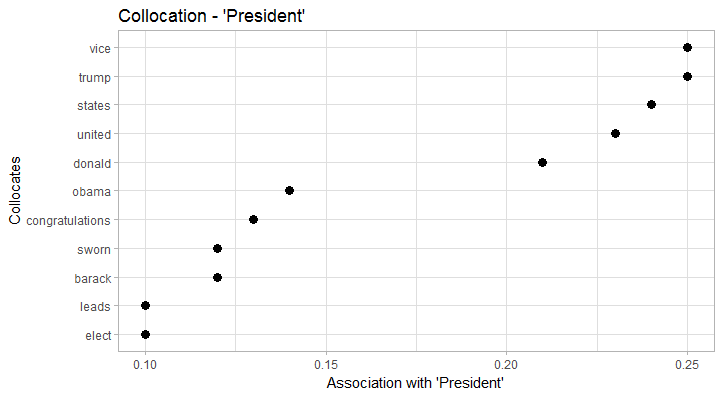
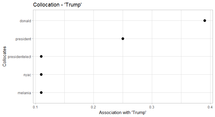
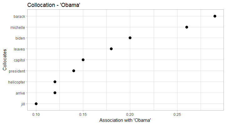
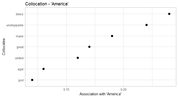
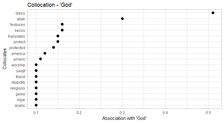
President collocates particularly strong with vice and trump. In terms of collocation strength, trump clearly trumps (…) obama as the new President. Also, we clearly see the formula President of the United States. Trump obviously collocates with donald (just as Obama collocates with barack), but also with presidentelect, president, nyac (New York Athletic Club), and melania. Obama on the other hand has a more diverse collocation profile that, for example, includes former Vice President biden. In both cases, the respective wives/First Ladies clearly collocate with ‘their’ President. America, in terms of collocates, seems to have a good run: it is depicted as unstoppable, great, united, and of course blessed by god (God bless America). This also explains the fairly high frequency of god in the data.

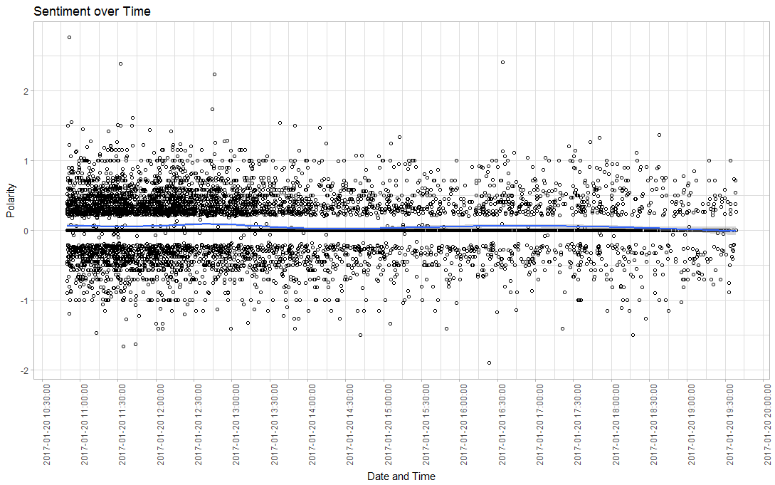
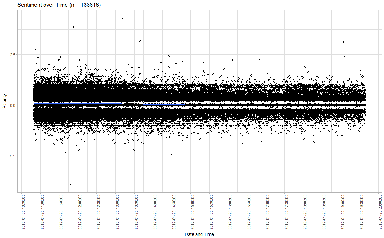
Sentiment Analysis

Plotting sentiment (polarity between -2/2; using the Hu and Liu (2004) dictionary) over time hints us towards three insights: Overall, the sentiment was balanced. However, the large spread in both directions at least indicates a divide between supporters and critics. Also we can observe that there were two (very minor) positive spikes in sentiment at around 12:30pm (Jackie Evancho performance) and 5pm (Parade).

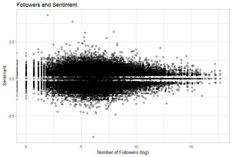
The following graph indicates that users with more followers may tend to write more neutral statuses. Calculating the Pearson correlation coefficient indicates a significant, but very weak relationship (p = .0177, r = 0.0065). This, however, needs to be investigated further.